Computing accurate eigenvalues using a mixed-precision Jacobi algorithm

Posted August 24, 2025

Nicholas J. Higham, François Tisseur, Marcus Webb, and I have uploaded to the arXiv our paper "Computing accurate eigenvalues using a mixed-precision Jacobi algorithm".

This paper builds on the famous result by Demmel and Veselić on the high accuracy of the Jacobi algorithm, in which they proved that for $A \in \mathbb{R}^{n\times n}$, if $\lambda_{k}(A)$ denotes the $k$-th largest exact eigenvalue of $A$ and $\widehat{\lambda}_{k}(A)$ is the $k$-th largest eigenvalue computed by the Jacobi algorithm with a suitable stopping criterion, then

\[\left| \frac{\widehat{\lambda}_{k}(A) - \lambda_{k}(A)}{\lambda_{k}(A)} \right| \le p(n)\,u\,\kappa_{2}^{S}(A), \]

where $p(n)$ is a low-degree polynomial, $u$ is the unit roundoff of the working precision, and $\kappa_{2}^{S}(A) = \sigma_{\max}(DAD)/\sigma_{\min}(DAD)$ with $D = \mathrm{diag}(a_{ii}^{-1/2})$.

Our algorithm

We first construct a preconditioner $\widetilde{Q}$ using either a spectral decomposition or a tridiagonal reduction computed at low precision. This preconditioner satisfies:

$\widetilde{Q}^{T}A\widetilde{Q}$ has small off-diagonal entries, and
$||\widetilde{Q}^{T}\widetilde{Q} - I||_{2}$ is of order $u$.

We then apply the Jacobi algorithm at working precision to $\widetilde{Q}^{T}A\widetilde{Q}$, which is evaluated at high precision. We refer to this approach as the mixed-precision preconditioned Jacobi algorithm.

Let $\widetilde{A} = \widetilde{Q}^{T}A\widetilde{Q}$. The eigenvalues computed by applying our algorithm to $\widetilde{A}$ satisfy

\[\left| \frac{\widehat{\lambda}_{k}(\widetilde{A}) - \lambda_{k}(A)}{\lambda_{k}(A)} \right| \le p(n)\,u\,\kappa_{2}^{S}(\widetilde{A}). \]

Through this procedure, $\kappa_{2}^{S}(A)$ is effectively replaced by $\kappa_{2}^{S}(\widetilde{A})$, which is often much smaller. For example, if $||A - \mathrm{diag}(A)||_F/\min_i(\widetilde{a}_{ii}) < 1/2$, then $\kappa_{2}^{S}(\widetilde{A}) < 3$.

Why high precision?

A key feature of our algorithm is the use of high-precision matrix–matrix multiplication. With sufficiently high precision, we can overcome the large componentwise forward errors that would otherwise arise when forming $\widetilde{Q}^{T}A\widetilde{Q}$.

Numerical Experiment

We compare four algorithms:
(a) MP2Jacobi -- our algorithm but with the matrix product $\widetilde{Q}^{T}A\widetilde{Q}$ evaluated at working precision,
(b) MP3Jacobi -- our proposed algorithm (matrix product evaluated at high precision),
(c) Jacobi -- the Jacobi algorithm of Demmel and Veselić, and
(d) MATLAB -- eig routine.

The test matrices are generated by:

gallery('randsvd', 100, -kappa, 5);

with condition numbers $\kappa$ varying from $10$ to $10^{16}$.

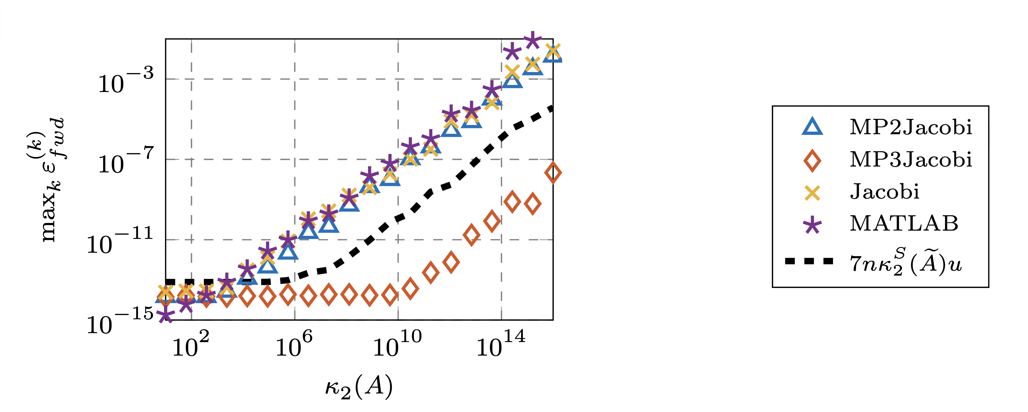
The results clearly show that our algorithm performs especially well for highly ill-conditioned matrices. For matrices with condition number $10^{16}$, MP3Jacobi achieves 7 correct digits of accuracy, whereas the other algorithms fail to reach 3 correct digits.